Jay Taylor's notes

How a Kalman filter works, in pictures | Bzarg

Clipped on: 2022-01-05

vec{x} = begin{bmatrix}
p
v
end{bmatrix}$$

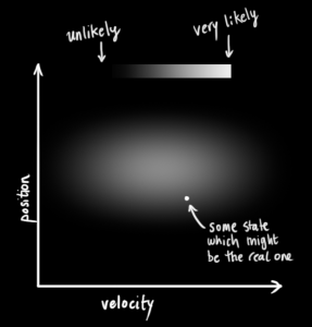
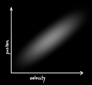
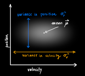
We don’t know what the actual position and velocity are; there are a whole range of possible combinations of position and velocity that might be true, but some of them are more likely than others:

begin{equation} label{eq:statevars}
begin{aligned}
mathbf{hat{x}}_k &= begin{bmatrix}
text{position}
text{velocity}
end{bmatrix}
mathbf{P}_k &=
begin{bmatrix}
Sigma_{pp} & Sigma_{pv}
Sigma_{vp} & Sigma_{vv}
end{bmatrix}
end{aligned}
end{equation}
$$

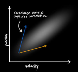
(Of course we are using only position and velocity here, but it’s useful to remember that the state can contain any number of variables, and represent anything you want).

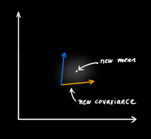
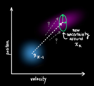
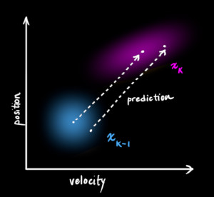
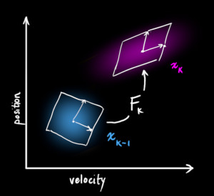
Next, we need some way to look at the current state (at time k-1) and predict the next state at time k. Remember, we don’t know which state is the “real” one, but our prediction function doesn’t care. It just works on all of them, and gives us a new distribution:

begin{split}
color{deeppink}{p_k} &= color{royalblue}{p_{k-1}} + Delta t &color{royalblue}{v_{k-1}}
color{deeppink}{v_k} &= &color{royalblue}{v_{k-1}}
end{split}
$$ In other words: $$
begin{align}
color{deeppink}{mathbf{hat{x}}_k} &= begin{bmatrix}
1 & Delta t
0 & 1
end{bmatrix} color{royalblue}{mathbf{hat{x}}_{k-1}}
&= mathbf{F}_k color{royalblue}{mathbf{hat{x}}_{k-1}} label{statevars}
end{align}
$$

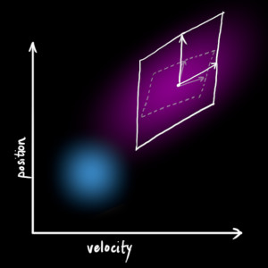
We now have a prediction matrix which gives us our next state, but we still don’t know how to update the covariance matrix.

This is where we need another formula. If we multiply every point in a distribution by a matrix (color{firebrick}{mathbf{A}}), then what happens to its covariance matrix (Sigma)?

Well, it’s easy. I’ll just give you the identity:$$
begin{equation}
begin{split}
Cov(x) &= Sigma
Cov(color{firebrick}{mathbf{A}}x) &= color{firebrick}{mathbf{A}} Sigma color{firebrick}{mathbf{A}}^T
end{split} label{covident}
end{equation}
$$

So combining (eqref{covident}) with equation (eqref{statevars}):$$
begin{equation}
begin{split}
color{deeppink}{mathbf{hat{x}}_k} &= mathbf{F}_k color{royalblue}{mathbf{hat{x}}_{k-1}}
color{deeppink}{mathbf{P}_k} &= mathbf{F_k} color{royalblue}{mathbf{P}_{k-1}} mathbf{F}_k^T
end{split}
end{equation}
$$

External influence

We haven’t captured everything, though. There might be some changes that aren’t related to the state itself— the outside world could be affecting the system.

For example, if the state models the motion of a train, the train operator might push on the throttle, causing the train to accelerate. Similarly, in our robot example, the navigation software might issue a command to turn the wheels or stop. If we know this additional information about what’s going on in the world, we could stuff it into a vector called (color{darkorange}{vec{mathbf{u}_k}}), do something with it, and add it to our prediction as a correction.

Let’s say we know the expected acceleration (color{darkorange}{a}) due to the throttle setting or control commands. From basic kinematics we get: $$
begin{split}
color{deeppink}{p_k} &= color{royalblue}{p_{k-1}} + {Delta t} &color{royalblue}{v_{k-1}} + &frac{1}{2} color{darkorange}{a} {Delta t}^2
color{deeppink}{v_k} &= &color{royalblue}{v_{k-1}} + & color{darkorange}{a} {Delta t}
end{split}
$$ In matrix form: $$
begin{equation}
begin{split}
color{deeppink}{mathbf{hat{x}}_k} &= mathbf{F}_k color{royalblue}{mathbf{hat{x}}_{k-1}} + begin{bmatrix}
frac{Delta t^2}{2}
Delta t
end{bmatrix} color{darkorange}{a}
&= mathbf{F}_k color{royalblue}{mathbf{hat{x}}_{k-1}} + mathbf{B}_k color{darkorange}{vec{mathbf{u}_k}}
end{split}
end{equation}
$$

(mathbf{B}_k) is called the control matrix and (color{darkorange}{vec{mathbf{u}_k}}) the control vector. (For very simple systems with no external influence, you could omit these).

Let’s add one more detail. What happens if our prediction is not a 100% accurate model of what’s actually going on?

External uncertainty

Everything is fine if the state evolves based on its own properties. Everything is still fine if the state evolves based on external forces, so long as we know what those external forces are.

But what about forces that we don’t know about? If we’re tracking a quadcopter, for example, it could be buffeted around by wind. If we’re tracking a wheeled robot, the wheels could slip, or bumps on the ground could slow it down. We can’t keep track of these things, and if any of this happens, our prediction could be off because we didn’t account for those extra forces.

We can model the uncertainty associated with the “world” (i.e. things we aren’t keeping track of) by adding some new uncertainty after every prediction step:

begin{equation}
begin{split}
color{deeppink}{mathbf{hat{x}}_k} &= mathbf{F}_k color{royalblue}{mathbf{hat{x}}_{k-1}} + mathbf{B}_k color{darkorange}{vec{mathbf{u}_k}}
color{deeppink}{mathbf{P}_k} &= mathbf{F_k} color{royalblue}{mathbf{P}_{k-1}} mathbf{F}_k^T + color{mediumaquamarine}{mathbf{Q}_k}
end{split}
label{kalpredictfull}
end{equation}
$$

In other words, the new best estimate is a prediction made from previous best estimate, plus a correction for known external influences.

And the new uncertainty is predicted from the old uncertainty, with some additional uncertainty from the environment.

All right, so that’s easy enough. We have a fuzzy estimate of where our system might be, given by (color{deeppink}{mathbf{hat{x}}_k}) and (color{deeppink}{mathbf{P}_k}). What happens when we get some data from our sensors?

Refining the estimate with measurements

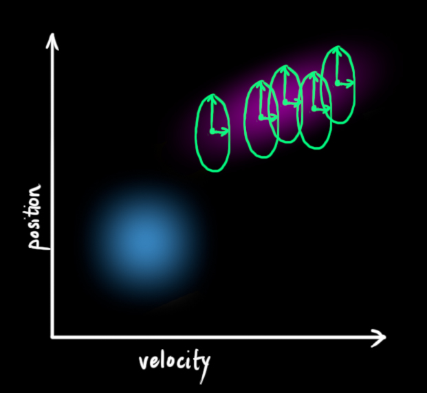
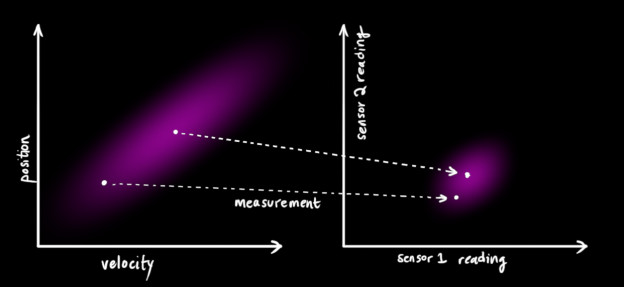
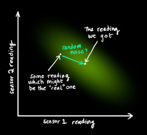
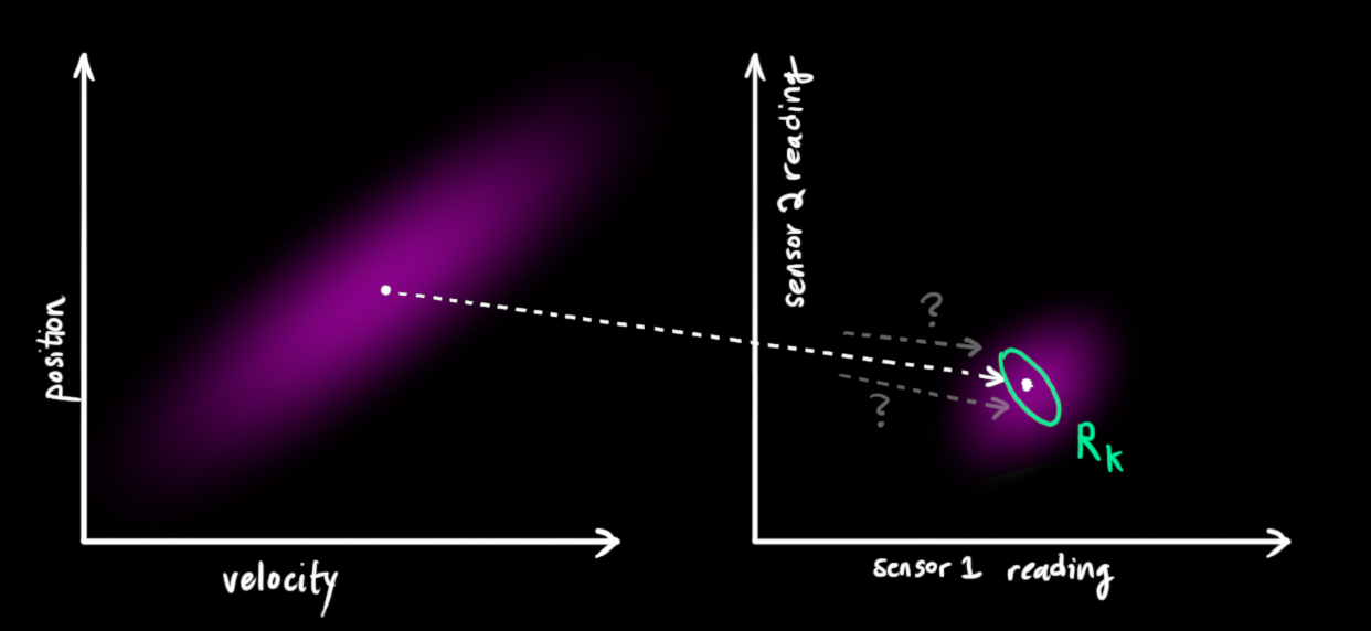
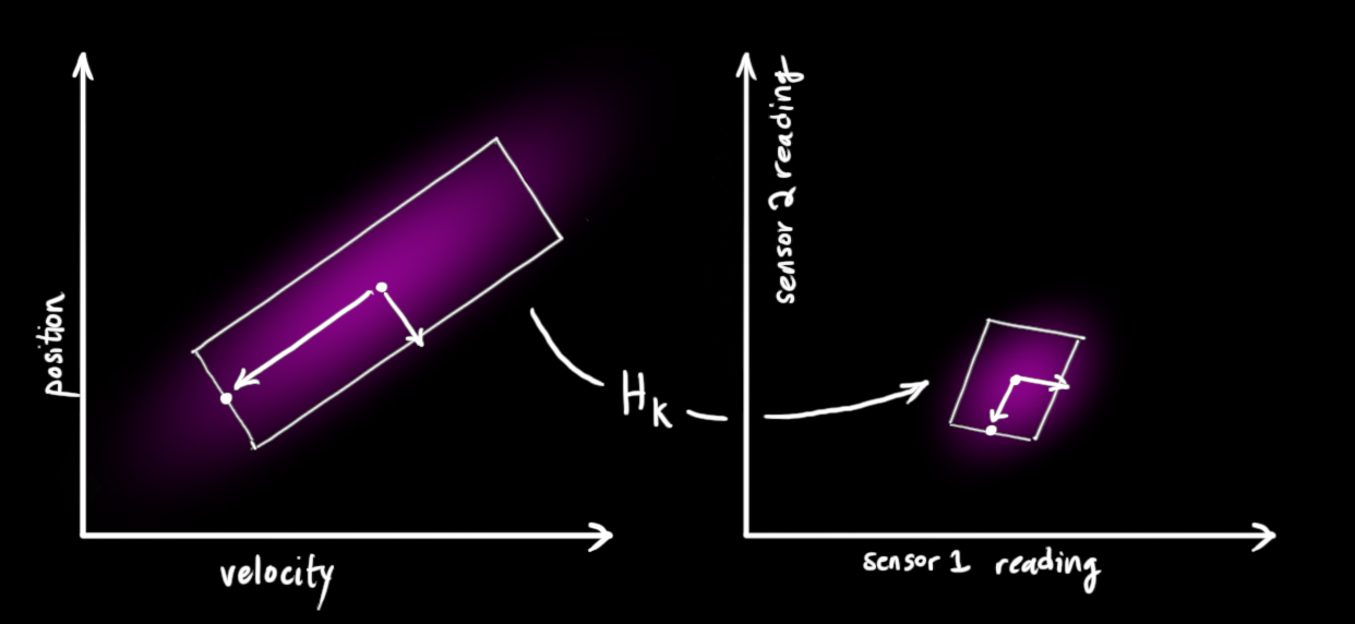
We might have several sensors which give us information about the state of our system. For the time being it doesn’t matter what they measure; perhaps one reads position and the other reads velocity. Each sensor tells us something indirect about the state— in other words, the sensors operate on a state and produce a set of readings.

begin{equation}
begin{aligned}
vec{mu}_{text{expected}} &= mathbf{H}_k color{deeppink}{mathbf{hat{x}}_k}
mathbf{Sigma}_{text{expected}} &= mathbf{H}_k color{deeppink}{mathbf{P}_k} mathbf{H}_k^T
end{aligned}
end{equation}
$$

One thing that Kalman filters are great for is dealing with sensor noise. In other words, our sensors are at least somewhat unreliable, and every state in our original estimate might result in a range of sensor readings. begin{equation} label{gaussformula}
mathcal{N}(x, mu,sigma) = frac{1}{ sigma sqrt{ 2pi } } e^{ -frac{ (x – mu)^2 }{ 2sigma^2 } }
end{equation}
$$

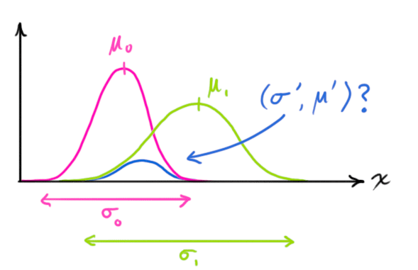
We want to know what happens when you multiply two Gaussian curves together. The blue curve below represents the (unnormalized) intersection of the two Gaussian populations:

mathcal{N}(x, color{fuchsia}{mu_0}, color{deeppink}{sigma_0}) cdot mathcal{N}(x, color{yellowgreen}{mu_1}, color{mediumaquamarine}{sigma_1}) stackrel{?}{=} mathcal{N}(x, color{royalblue}{mu’}, color{mediumblue}{sigma’})
end{equation}$$

You can substitute equation (eqref{gaussformula}) into equation (eqref{gaussequiv}) and do some algebra (being careful to renormalize, so that the total probability is 1) to obtain: $$
begin{equation} label{fusionformula}
begin{aligned}
color{royalblue}{mu’} &= mu_0 + frac{sigma_0^2 (mu_1 – mu_0)} {sigma_0^2 + sigma_1^2}
color{mediumblue}{sigma’}^2 &= sigma_0^2 – frac{sigma_0^4} {sigma_0^2 + sigma_1^2}
end{aligned}
end{equation}$$

We can simplify by factoring out a little piece and calling it (color{purple}{mathbf{k}}): $$
begin{equation} label{gainformula}
color{purple}{mathbf{k}} = frac{sigma_0^2}{sigma_0^2 + sigma_1^2}
end{equation} $$ $$
begin{equation}
begin{split}
color{royalblue}{mu’} &= mu_0 + &color{purple}{mathbf{k}} (mu_1 – mu_0)
color{mediumblue}{sigma’}^2 &= sigma_0^2 – &color{purple}{mathbf{k}} sigma_0^2
end{split} label{update}
end{equation} $$

Take note of how you can take your previous estimate and add something to make a new estimate. And look at how simple that formula is!

But what about a matrix version? Well, let’s just re-write equations (eqref{gainformula}) and (eqref{update}) in matrix form. If (Sigma) is the covariance matrix of a Gaussian blob, and (vec{mu}) its mean along each axis, then: $$
begin{equation} label{matrixgain}
color{purple}{mathbf{K}} = Sigma_0 (Sigma_0 + Sigma_1)^{-1}
end{equation} $$ $$
begin{equation}
begin{split}
color{royalblue}{vec{mu}’} &= vec{mu_0} + &color{purple}{mathbf{K}} (vec{mu_1} – vec{mu_0})
color{mediumblue}{Sigma’} &= Sigma_0 – &color{purple}{mathbf{K}} Sigma_0
end{split} label{matrixupdate}
end{equation}
$$

(color{purple}{mathbf{K}}) is a matrix called the Kalman gain, and we’ll use it in just a moment.

Easy! We’re almost finished!

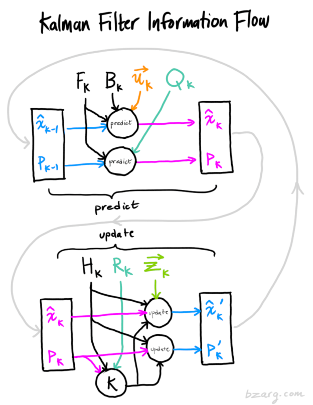
Putting it all together

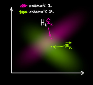
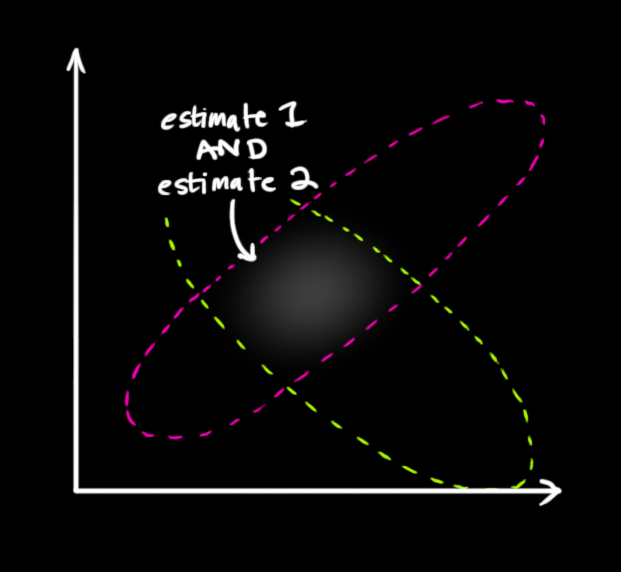
We have two distributions: The predicted measurement with ( (color{fuchsia}{mu_0}, color{deeppink}{Sigma_0}) = (color{fuchsia}{mathbf{H}_k mathbf{hat{x}}_k}, color{deeppink}{mathbf{H}_k mathbf{P}_k mathbf{H}_k^T}) ), and the observed measurement with ( (color{yellowgreen}{mu_1}, color{mediumaquamarine}{Sigma_1}) = (color{yellowgreen}{vec{mathbf{z}_k}}, color{mediumaquamarine}{mathbf{R}_k})). We can just plug these into equation (eqref{matrixupdate}) to find their overlap: $$
begin{equation}
begin{aligned}
mathbf{H}_k color{royalblue}{mathbf{hat{x}}_k’} &= color{fuchsia}{mathbf{H}_k mathbf{hat{x}}_k} & + & color{purple}{mathbf{K}} ( color{yellowgreen}{vec{mathbf{z}_k}} – color{fuchsia}{mathbf{H}_k mathbf{hat{x}}_k} )
mathbf{H}_k color{royalblue}{mathbf{P}_k’} mathbf{H}_k^T &= color{deeppink}{mathbf{H}_k mathbf{P}_k mathbf{H}_k^T} & – & color{purple}{mathbf{K}} color{deeppink}{mathbf{H}_k mathbf{P}_k mathbf{H}_k^T}
end{aligned} label {kalunsimplified}
end{equation}
$$ And from (eqref{matrixgain}), the Kalman gain is: $$
begin{equation} label{eq:kalgainunsimplified}
color{purple}{mathbf{K}} = color{deeppink}{mathbf{H}_k mathbf{P}_k mathbf{H}_k^T} ( color{deeppink}{mathbf{H}_k mathbf{P}_k mathbf{H}_k^T} + color{mediumaquamarine}{mathbf{R}_k})^{-1}
end{equation}
$$ We can knock an (mathbf{H}_k) off the front of every term in (eqref{kalunsimplified}) and (eqref{eq:kalgainunsimplified}) (note that one is hiding inside (color{purple}{mathbf{K}}) ), and an (mathbf{H}_k^T) off the end of all terms in the equation for (color{royalblue}{mathbf{P}_k’}). $$
begin{equation}
begin{split}
color{royalblue}{mathbf{hat{x}}_k’} &= color{fuchsia}{mathbf{hat{x}}_k} & + & color{purple}{mathbf{K}’} ( color{yellowgreen}{vec{mathbf{z}_k}} – color{fuchsia}{mathbf{H}_k mathbf{hat{x}}_k} )
color{royalblue}{mathbf{P}_k’} &= color{deeppink}{mathbf{P}_k} & – & color{purple}{mathbf{K}’} color{deeppink}{mathbf{H}_k mathbf{P}_k}
end{split}
label{kalupdatefull}
end{equation} $$ $$
begin{equation}
color{purple}{mathbf{K}’} = color{deeppink}{mathbf{P}_k mathbf{H}_k^T} ( color{deeppink}{mathbf{H}_k mathbf{P}_k mathbf{H}_k^T} + color{mediumaquamarine}{mathbf{R}_k})^{-1}
label{kalgainfull}
end{equation}
$$ …giving us the complete equations for the update step.

And that’s it! (color{royalblue}{mathbf{hat{x}}_k’}) is our new best estimate, and we can go on and feed it (along with ( color{royalblue}{mathbf{P}_k’} ) ) back into another round of predict or update as many times as we like.

Some credit and referral should be given to this fine document, which uses a similar approach involving overlapping Gaussians. More in-depth derivations can be found there, for the curious.

How can I plot the uncertainty surrounding each point (mean) in python?

Reply ↓

M = [m11, m12; m21, m22]
u = [u1; u2]
your x and y values would be
x = u1 + m11 * cos(theta) + m12 * sin(theta)
y = u2 + m21 * cos(theta) + m22 * sin(theta)
Just sweep theta from 0 to 2pi and you’ve got an ellipse!

For a more in-depth approach check out this link:
https://www.visiondummy.com/2014/04/draw-error-ellipse-representing-covariance-matrix/

Thanks.

Reply ↓

https://www.bzarg.com/wp-content/uploads/2015/08/kalflow.png

Reply ↓
1. I wish I’d known about these filters a couple years back – they would have helped me solve an embedded control problem with lots of measurement uncertainty.
  
  Thanks for the great post!
  
  Reply ↓
2. – observed noisy mean and covariance (z and R) we want to correct, and
  – an additional info ‘control vector’ (u) with known relation to our prediction.
  Correct?
  
  Does H in (8) maps physical measurements (e.g. km/h) into raw data readings from sensors (e.g. uint32, as described in some accelerometer’s reference manual)?
  
  Reply ↓
  1. However, I still do not have an understanding of what APA^T is doing and how it is different from AP.
    
    Reply ↓
I guess the same thing applies to equation right before (6)?

Regards,
Istvan Hajnal

Reply ↓
1. Regards,
  Li
  
  Reply ↓
  1. https://math.stackexchange.com/q/2630447
    
    Reply ↓

I think this operation is forbidden for this matrix.

Reply ↓

Can anyone help me with this?

Reply ↓

thank you very much

Reply ↓

There is no doubt, this is the best tutorial about KF !
Many thanks!

Reply ↓

Thanks Baljit

Reply ↓

on point….and very good work…..

Reply ↓

Equation 16 is right. Divide all by H.

Reply ↓

z has the units of the measurement variables.
K is unitless 0-1.
The units don’t work unless the right term is K(z/H-x).

Reply ↓
I want to use kalman Filter to auto correct 2m temperature NWP forecasts.
Could you please help me to get a solution or code in R, FORTRAN or Linux Shell Scripts(bash,perl,csh,…) to do this.

Reply ↓
I’m kinda new to this field and this document helped me a lot
I just have one question and that is what is the value of the covariance matrix at the start of the process?

Reply ↓
Thanks.

Reply ↓
I had to laugh when I saw the diagram though, after seeing so many straight academic/technical flow charts of this, this was refreshing :D

If anyone really wants to get into it, implement the formulas in octave or matlab then you will see how easy it is. This filter is extremely helpful, “simple” and has countless applications.

Reply ↓
great article.
there is a typo in eq(13) which should be sigam_1 instead of sigma_0.

Reply ↓
1. sometimes the easiest way to explain something is really the harthest!
  You did it!
  
  Reply ↓
  1. This is where we need another formula. If we multiply every point in a distribution by a matrix A, then what happens to its covariance matrix Σ?
    
    Well, it’s easy. I’ll just give you the identity:
    Cov(x)=Σ
    Cov(Ax)==AΣA^T
    “””
    
    Why is that easy? Thanks so much for your effort!
    
    Reply ↓
    1. — you spread state x out by multiplying by A
      — sigma is the covariance of the vector x (1d), which spreads x out by multiplying x by itself into 2d
      so
      — you spread the covariance of x out by multiplying by A in each dimension ; in the first dimension by A, and in the other dimension by A_t
      
      Reply ↓
  2. but i have a question please !
    why this ??
    We can knock an Hk off the front of every term in (16) and (17) (note that one is hiding inside K ), and an HTk off the end of all terms in the equation for P′k.
    
    Reply ↓
  3. it seems a C++ implementation of a Kalman filter is made here :
    https://github.com/hmartiro/kalman-cpp
    
    Reply ↓
  4. In equation (16), Where did the left part come from? Updated state is already multiplied by measurement matrix and knocked off? I couldn’t understand this step.
    
    Reply ↓
  5. A great refresher…
    
    Reply ↓
  6. One question:
    what exactly does H do? Can you give me an example of H? I was assuming that the observation x IS the mean of where the real x could be, and it would have a certain variance. But instead, the mean is Hx. Why is that? why is the mean not just x?
    Thanks!
    
    Reply ↓
  7. I have acceleration measurements only.How do I estimate position and velocity?
    What will be my measurement matrix?
    Is it possible to construct such a filter?
    
    Reply ↓
  8. What if the sensors don’t update at the same rate? You want to update your state at the speed of the fastest sensor, right? Do you “simply” reduce the rank of the H matrix for the sensors that haven’t been updated since the last prediction?
    
    Reply ↓
  9. Could you pleaseeeee extend this to the Extended, Unscented and Square Root Kalman Filters as well.
    
    Reply ↓
  10. Really a great one, I loved it!
    
    Reply ↓
  11. Thanks
    
    Reply ↓
  12. ‘The Extended Kalman Filter: An Interactive Tutorial for Non-Experts’
    https://home.wlu.edu/~levys/kalman_tutorial/
    (written to be understood by high-schoolers)
    
    Reply ↓
  13. And did I mention you are brilliant!!!? :-)
    
    Reply ↓
Thanks for your effort

Reply ↓
hope the best for you ^_^

Reply ↓
Krishna

Reply ↓
1. i need to implémet a banc of 4 observers (kalman filter) with DOS( Dedicated observer), in order to detect and isolate sensors faults
  each observer is designed to estimate the 4 system outputs qu’une seule sortie par laquelle il est piloté, les 3 autres sorties restantes ne sont pas bien estimées, alors que par définition de la structure DOS, chaque observateur piloté par une seule sortie et toutes les entrées du système doit estimer les 4 sorties.
  SVP veuillez m’indiquer comment faire pour résoudre ce problème et merci d’avance
  
  Reply ↓
2. Thank you very much.
  
  But I still have a question, why use multiply to combine Gaussians?
  Maybe it is too simple to verify.
  
  Reply ↓
3. Can you please explain:
  1. How do we initialize the estimator ?
  2. How does the assumption of noise correlation affects the equations ?
  3. How can we see this system is linear (a simple explanation with an example like you did above would be great!) ?
  
  Reply ↓
4. first get the mean as: mean(x)=sum(xi)/n
  then the variance is given as: var(x)=sum((xi-mean(x))^2)/n
  see here (scroll down for discrete equally likely values): https://en.wikipedia.org/wiki/Variance
  
  Cheers,
  Romain
  
  Reply ↓
  1. Aditya
    
    Reply ↓
  2. Thank you so much :)
    
    Reply ↓
  3. What is Hk exactly, what if my mobile have two sensors for speed for example and one very noisy for position…
    
    Reply ↓
  4. FINALLY found THE article that clear things up!
    Thanks for the awesome article!
    
    Reply ↓
  5. By the way, can I translate this blog into Chinese? Of course, I will put this original URL in my translated post. :)
    
    Reply ↓
  6. I am still curious about examples of control matrices and control vectors – the explanation of which you were kind enough to gloss over in this introductory exposition.
    I have a lot of other questions and any help would be appreciated!
    I have a strong background in stats and engineering math and I have implemented K Filters and Ext K Filters and others as calculators and algorithms without a deep understanding of how they work. I would like to get a better understanding please with any help you can provide. Thank you!
    
    Reply ↓
  7. yes i can use the coordinates ( from sensor/LiDAR ) of first two frame to find the velocity but that is again NOT completely reliable source
    
    what should i do???
    
    Reply ↓
  8. If we’re trying to get xk, then shouldn’t xk be computed with F_k-1, B_k-1 and u_k-1? It is because, when we’re beginning at an initial time of k-1, and if we have x_k-1, then we should be using information available to use for projecting ahead…. which means F_k-1, B_k-1 and u_k-1, right? Not F_k, B_k and u_k.
    
    Reply ↓
    1. x[k+1] = Ax[k] + Bu[k]. I assumed that A is Ak, and B is Bk.
      Then, when re-arranging the above, we get:
      x[k] = Ax[k-1] + Bu[k-1]. I assumed here that A is A_k-1 and B is B_k-1. This suggests order is important. But, on the other hand, as long as everything is defined …. then that’s ok. Thanks again! Nice site, and nice work.
      
      Reply ↓
5. Thanks in advance.
  
  Reply ↓
6. I think I need read it again,
  Explanation of Kalman Gain is superb.
  Thanks a lot
  
  Reply ↓
7. I really would like to read a follow-up about Unscented KF or Extended KF from you.
  
  Reply ↓
8. Can someone be kind enough to explain that part to me ? How do you normalize a Gaussian distribution ? Sorry for the newby question, trying to undertand the math a bit.
  
  Thanks in advance
  
  Reply ↓
  1. Joseph Cluever February 14, 2018 at 6:17 pm
    
    The integral of a distribution over it’s domain has to be 1 by definition. Also, I don’t know if that comment in the blog is really necessary because if you have the covariance matrix of a multivariate normal, the normalizing constant is known: det(2*pi*(Covariance Matrix))^(-1/2). There’s nothing to really be careful about. See https://en.wikipedia.org/wiki/Multivariate_normal_distribution
    
    Reply ↓
9. Nathaniel Groendyk February 9, 2018 at 1:50 am
  
  Amazing article! Very impressed! You must have spent some time on it, thank you for this!
  
  I had one quick question about Matrix H. Can it be extended to have more sensors and states? For example say we had 3 sensors, and the same 2 states, would the H matrix look like this:
  H = [ [Sensor1-to-State 1(vel) conversion Eq , Sensor1-to-State 2(pos) conversion Eq ] ;
  [Sensor2-to-State 1(vel) conversion Eq , Sensor2-to-State 2(pos) conversion Eq ] ;
  [Sensor3-to-State 1(vel) conversion Eq , Sensor3-to-State 2(pos) conversion Eq ] ]
  
  Thank you!
  
  Reply ↓
10. Sasanka Kuruppuarachchi February 21, 2018 at 5:44 am
  
  Simply love it.
  
  Reply ↓
11. hamza February 23, 2018 at 9:54 am
  
  Hey Author,
  Good work. Can you elaborate how equation 4 and equation 3 are combined to give updated covariance matrix?
  
  Reply ↓
  1. tbabb Post authorFebruary 23, 2018 at 7:51 pm
    
    (F_k) is a matrix applied to a random vector (x_{k-1}) with covariance (P_{k-1}). Equation (4) says what we do to the covariance of a random vector when we multiply it by a matrix.
    
    Reply ↓
12. Ankit Swarnkar February 27, 2018 at 9:22 pm
  
  Simply Awesome!
  
  Reply ↓
13. Sangyun Han March 6, 2018 at 1:35 am
  
  This article is the best one about Kalman filter ever. Thanks for your help.
  
  But I have a question about how to do knock off Hk in equation (16), (17).
  Because usual case Hk is not invertible matrix, so i think knocking off Hk is not possible.
  Can you explain?
  
  Reply ↓
14. Dasarath S March 7, 2018 at 1:19 pm
  
  Mind Blown !! The fact that you perfectly described the reationship between math and real world is really good. Thnaks a lot!!
  
  Reply ↓
15. P P BANERJEE March 10, 2018 at 7:42 pm
  
  Can this method be used accurately to predict the future position if the movement is random like Brownian motion.
  
  Reply ↓
  1. tbabb Post authorMarch 12, 2018 at 6:02 pm
    
    If you have sensors or measurements providing some current information about the position of your system, then sure.
    
    In the case of Brownian motion, your prediction step would leave the position estimate alone, and simply widen the covariance estimate with time by adding a constant (Q_k) representing the rate of diffusion. Your measurement update step would then tell you to where the system had advanced.
    
    Reply ↓
16. Lorenzo March 13, 2018 at 10:24 am
  
  It is an amazing article, thank you so much for that!!!!!
  
  Reply ↓
17. salma rv March 17, 2018 at 6:28 am
  
  Is the method useful for biological samples variations from region to region
  
  Reply ↓
18. João Escusa March 21, 2018 at 12:05 pm
  
  Hello.
  
  I’m trying to implement a Kalman filter for my thesis ut I’ve never heard of it and have some questions.
  I save the GPS data of latitude, longitude, altitude and speed. So my position is not a variable, so to speak, it’s a state made of 4 variables if one includes the speed. Data is acquired every second, so whenever I do a test I end up with a large vector with all the information.
  
  How does one calculate the covariance and the mean in this case? Probabilities have never been my strong suit.
  
  Thanks.
  
  Reply ↓
  1. tbabb Post authorMarch 22, 2018 at 2:17 am
    
    Take many measurements with your GPS in circumstances where you know the “true” answer. This will produce a bunch of state vectors, as you describe. Find the difference of these vectors from the “true” answer to get a bunch of vectors which represent the typical noise of your GPS system. Then calculate the sample covariance on that set of vectors. That will give you (R_k), the sensor noise covariance.
    
    You can estimate (Q_k), the process covariance, using an analogous process.
    
    Note that to meaningfully improve your GPS estimate, you need some “external” information, like control inputs, knowledge of the process which is moving your vehicle, or data from other, separate inertial sensors. Running Kalman on only data from a single GPS sensor probably won’t do much, as the GPS chip likely uses Kalman internally anyway, and you wouldn’t be adding anything!
    
    Reply ↓
19. Yar Zar April 28, 2018 at 7:50 am
  
  Well explanation! Thank you so much!
  
  Reply ↓
20. Vladimir May 7, 2018 at 8:19 pm
  
  Many thanks!
  I’ve never seen such a clear and passionate explanation.
  
  Reply ↓
21. Di May 17, 2018 at 3:38 am
  
  Excellent explanation. Thank you!
  
  Reply ↓
22. P February 23, 2019 at 3:43 pm
  
  Great tutorial! Thanks! :D
  
  Reply ↓
23. Grant March 14, 2019 at 11:16 pm
  
  FANTASTIC explanation! Just EPIC:-)
  
  Reply ↓
24. Steve March 20, 2019 at 9:50 am
  
  Agree with Grant, this is a fantastic explanation, please do your piece on extended KF’s – non linear systems is what I’m looking at!!
  
  Reply ↓
25. modar March 25, 2019 at 4:35 pm
  
  Perfect ,easy and insightful explanation; thanks a lot.
  
  Reply ↓
26. Eranga De Silva April 3, 2019 at 3:35 am
  
  Thank you VERY much for this nice and clear explanation
  
  Reply ↓
27. Will April 27, 2019 at 2:28 am
  
  That was an amazing post! Thank you so much for the wonderful explanation!
  
  As a side note, the link in the final reference is no longer up-to-date. Now it seems this is the correct link: https://drive.google.com/file/d/1nVtDUrfcBN9zwKlGuAclK-F8Gnf2M_to/view
  
  Once again, congratz on the amazing post!
  
  Reply ↓
28. cle323 May 16, 2019 at 4:41 am
  
  THANK YOU !!
  
  After spending 3 days on internet, I was lost and confused. Your explanation is very clear ! Nice job
  
  Reply ↓
29. Richard May 26, 2019 at 4:59 pm
  
  This was very clear until I got to equation 5 where you introduce P without saying what is it and how its prediction equation relates to multiplying everything in a covariance matrix by A.
  
  Reply ↓
30. Richard May 26, 2019 at 5:06 pm
  
  Sorry, ignore previous comment. I’ve traced back and found it.
  
  Reply ↓
31. 孙凯道 May 30, 2019 at 10:22 am
  
  THANK YOU
  Such a meticulous post gave me a lot of help.
  
  Reply ↓
32. Monty June 15, 2019 at 2:44 am
  
  So it seems it’s interpolating state from prediction and state from measurement. H x_meas = z. Doesn’t seem like x_meas is unique.
  
  Reply ↓
33. Maxim July 16, 2019 at 12:34 pm
  
  Thanks for the post.
  I still have few questions.
  
  1. At eq. (5) you put evolution as a motion without acceleration. At eq. 5 you add acceleration and put it as some external force. But it is not clear why you separate acceleration, as it is also a part of kinematic equation. So, the question is what is F and what is B. Can/should I put acceleration in F?
  
  2. At eq. 7 you update P with F, but not with B, despite the x is updated with both F & B. Why?
  
  Reply ↓
  1. tbabb Post authorJuly 16, 2019 at 5:32 pm
    
    1. The state of the system (in this example) contains only position and velocity, which tells us nothing about acceleration. F is a matrix that acts on the state, so everything it tells us must be a function of the state alone. If our system state had something that affected acceleration (for example, maybe we are tracking a model rocket, and we want to include the thrust of the engine in our state estimate), then F could both account for and change the acceleration in the update step. Otherwise, things that do not depend on the state x go in B.
    
    2. P represents the covariance of our state— how the possibilities are balanced around the mean. B affects the mean, but it does not affect the balance of states around the mean, so it does not matter in the calculation of P. This is because B does not depend on the state, so adding B is like adding a constant, which does not distort the shape of the distribution of states we are tracking.
    
    Reply ↓
34. Abdul Basit July 17, 2019 at 12:25 am
  
  Great intuition, I am bit confuse how Kalman filter works. But this blog clear my mind and I am able to understand Computer Vision Tracking algorithms.
  
  Reply ↓
35. Monty August 22, 2019 at 8:16 am
  
  My issue is with you plucking H’s off of this:
  H x’ = H x + H K (z – H x)
  x’ = x + K (z – H x) <- we know this is true from a more rigorous derivation
  
  H isn't generally invertible. For sure you can go the other way by adding H back in. However, I do like this explaination.
  
  Reply ↓
36. Abdelrhman September 20, 2019 at 4:17 pm
  
  Thanks alot for this, it’s really the best explanation i’ve seen for the Kalman filter. visualization with the idea of merging gaussians for the correction/update step and to find out where the kalman gain “K” came from is very informative.
  
  Reply ↓
37. Kimon September 23, 2019 at 9:45 pm
  
  Is there a way to combine sensor measurements where each of the sensors has a different latency? How does one handle that type of situation?
  
  Reply ↓
38. David Sorcman October 16, 2019 at 7:56 am
  
  This is the best explanation of KF that I have ever seen, even after graduate school.
  
  Just a warning though – in Equation 10, the “==?” should be “not equals” – the product of two Gaussians is not a Gaussian. See http://mathworld.wolfram.com/NormalProductDistribution.html for the actual distribution, which involves the Ksub0 Bessel function. The expressions for the variance are correct, but not the implication about the pdf.
  
  Also, since position has 3 components (one each along the x, y, and z axes), and ditto for velocity, the actual pdf becomes even more complicated. See the above link for the pdf for details in the 3 variable case.
  
  Reply ↓
  1. tbabb Post authorNovember 1, 2019 at 12:00 am
    
    See my other replies above: The product of two Gaussian PDFs is indeed a Gaussian. The PDF of the product of two Gaussian-distributed variables is the distribution you linked. For this application we need the former; the probability that two random independent events are simultaneously true.
    
    Reply ↓
39. Arye November 12, 2019 at 8:23 am
  
  Great Article!
  I have some questions: Where do I get the Qk and Rk from? Do I model them? How do I update them?
  Thanks!
  
  Reply ↓
40. Mariana Jimenez November 18, 2019 at 6:15 pm
  
  Thank you very much ! Great article
  I’ve been struggling a lot to understand the KF and this has given me a much better idea of how it works.
  
  Reply ↓
41. Ryder November 21, 2019 at 6:15 pm
  
  There’s a few things that are contradiction to what this paper https://arxiv.org/abs/1710.04055 says about Kalman filtering:
  
  “The Kalman filter assumes that both variables (postion and velocity, in our case) are random and Gaussian distributed”
  – Kalman filter only assumes that both variables are uncorrelated (which is a weaker assumption that independent). Kalman filters can be used with variables that have other distributions besides the normal distribution
  
  “In the above picture, position and velocity are uncorrelated, which means that the state of one variable tells you nothing about what the other might be.”
  – I think this a better description of what independence means that uncorrelated. Again, check out p. 13 of the Appendix of the reference paper by Y Pei et Al.
  
  Reply ↓
42. Dmitry November 22, 2019 at 2:05 am
  
  Great article, finally I got understanding of the Kalman filter and how it works.
  
  Reply ↓
43. Vlad February 14, 2020 at 12:49 am
  
  This was such a great article. Really good job!
  
  Reply ↓
44. Nishant Jain February 21, 2020 at 8:30 pm
  
  How do we get Qk and Hk matrices?
  
  Reply ↓
45. Yiding Yang March 4, 2020 at 9:06 am
  
  This is an amazing tutorial. Thanks!
  
  Reply ↓
46. Lepper April 7, 2020 at 3:06 am
  
  I have one question regarding state vector; what is the position? i would say it is [x, y, v], right? in this case how looks the prediction matrix? thanks!
  
  Reply ↓
47. Oussama April 14, 2020 at 8:48 pm
  
  Thanks, I think it was simple and cool as an introduction of KF
  
  really appreciate reading it
  
  Reply ↓
48. Om Kulkarni May 15, 2020 at 10:44 am
  
  I stumbled upon this article while learning autonomous mobile robots and I am completely blown away by this. The fact that an algorithm which I first thought was so boring could turn out to be so intuitive is just simply breathtaking.
  
  Thank you for this article and I hope to be a part of many more.
  
  Reply ↓
49. Diego May 21, 2020 at 11:11 am
  
  Hi ,
  I have never seen a very well and simple explanation as yours . It is amazing thanks a lot.
  I have a question ¿ How can I get Q and R Matrix ?
  
  Thanks again.
  
  Reply ↓
50. David Bellomo May 22, 2020 at 3:49 pm
  
  This tool is one of my cornerstones for my Thesis, I have beeing struggling to understand the math behind this topic for more thant I whish. Your article is just amazing, shows the level of mastery you have on the topic since you can bring the maths an a level that is understandable by anyone. This is a tremendous boost to my Thesis, I cannot thank you enough for this work you did.
  
  Reply ↓
51. Narendiran Chembu June 5, 2020 at 7:38 am
  
  Amazing Job. Thank you! :)
  
  Reply ↓
52. Diego Burgos August 7, 2020 at 2:27 pm
  
  Hi, thanks in advance for such a good post, I want to ask you how you deduce the equation (5) given (4), I will stick to your answer.
  
  Reply ↓
53. Rajat Mehta August 25, 2020 at 4:33 am
  
  One of the best intuitive explanation for Kalman Filter. Thanks for the amazing post.
  
  Reply ↓
54. Frederick C. Monson, PhD August 25, 2020 at 3:31 pm
  
  In the first set in a SEM I worked, there was button for a “Kalman” image adjustment. No one could explain what it was doing. Now, in the absence of calculous, I can present SEM users to use this help.
  
  Reply ↓
55. eya September 14, 2020 at 12:22 pm
  
  thank you it is very clear and helpful
  
  Reply ↓
56. Francisca October 20, 2020 at 8:33 pm
  
  I Loved how you used the colors!!! Very clear thank yoy
  
  Reply ↓
57. Hojae November 9, 2020 at 5:54 pm
  
  Thank you. it helps me a lot.
  
  Reply ↓
58. T. K. Prasad November 19, 2020 at 11:34 am
  
  Excellent blog!
  
  Reply ↓
59. YT Tseng January 1, 2021 at 7:20 pm
  
  Thank you tbabb! It is a very nice tutorial!
  I have a question.
  
  In equation15, you demonstrated the multiplication of the following two Gaussian distribution:
  mu_0 = Hk Xk_hat
  sigma_0 = Hk Pk Hk^T
  and
  mu_1 = zk
  sigma_1 = Rk
  
  but how can we interpret the two Gaussian distribution in probability form?
  should it be like this (x is for state, and y is for observed value)?
  P(xt|y1, …, yt-1)*P(yt|xt) = P(xt, yt|y1, y2, …, yt-1) as N~(mu_0, sigma_0)
  and
  P(??|??) as N~(mu_1, sigma_1)
  so that after multiplication (correction step), we get P(xt|y1, y2, …, yt)?
  Especially the probability form of the observed distribution confuses me.
  
  Looking forward to hearing from you. Happy new year!
  
  Reply ↓
60. William Gao January 14, 2021 at 12:20 am
  
  Thanks! That’s easy-understanding and interesting.
  
  Reply ↓
61. Mohammad Rahmani January 17, 2021 at 8:53 am
  
  I wish you had somethinf for particle filter too. Thanks anyway
  
  Reply ↓
62. Big Lebowsky March 6, 2021 at 2:40 am
  
  Thanks very good article actually helped me to finetune my python script to check K calculations in gravity.
  
  Reply ↓
63. Pedro Golmayo July 14, 2021 at 11:25 am
  
  Excellent. Thanks
  
  Reply ↓
64. Chen Chiyu August 7, 2021 at 8:39 pm
  
  Pictures are so cute
  
  Reply ↓
65. Chiyu Chen August 8, 2021 at 6:54 am
  
  Your pictures are all exquisite ! It is so cute to explain how a Kalman Filter works.
  
  Reply ↓
66. Tan Phan August 11, 2021 at 12:10 pm
  
  This is the best article that explains the topic interestingly.
  
  Reply ↓
67. ravi August 29, 2021 at 4:31 am
  
  Excellent article for understanding of kalman filter.. Thank you for explaining it beautifully
  
  Reply ↓
68. Amrit Sahu September 5, 2021 at 7:25 am
  
  One hell of an article. Awesome!!
  
  Reply ↓
69. Fitwi November 3, 2021 at 9:30 am
  
  Thank you for this article. It explains a lot. Keep up the good work.
  
  Reply ↓
70. mehmet rıza öz November 10, 2021 at 5:56 am
  
  Thank you for explaining all the cycle without any missing point.
  I could not understand them until reading your article.
  Great job!
  
  Reply ↓
71. Viiresh Yang November 19, 2021 at 4:40 am
  
  Great job! I really get benefit from this article.
  Thank you!
  
  Reply ↓
Leave a Reply
Your email address will not be published. Required fields are marked *
Comment
Name *

Email *

Website